Do you want to combine exports of two different Teamleader Focus modules in one Excel file? If you have a common column in both exports, you can put information from the one file into the other one. This requires some magic with the VLookup function in Excel. In this article we will discuss some use cases, the procedure and possible challenges.
And don't worry, you got this! It might seem complicated at the beginning, but once you run through the steps, it is pretty self-explanatory.
Use cases
Here you will find some examples of the Teamleader Focus possibilities regarding the VLookup function:
- You want extensive information about the related company in the contact export: use the common column 'Company name' (Export companies and exports contacts)
- In your invoice export you also want to see a custom field on product level: use the common column 'Product ID or Product name' (Export invoices and export products)
- When exporting your deals, you want detailed project information in your Excel: use the common column 'Project name' (Export deals and export projects)
- A more challenging example: You have two files you want to import, one with calls and one with customers. You only want to import the customers, however, for which you need to import calls: use the common column 'Customer name'. Here you will have to insert another 'trick'. Put an extra column in the call file with for each row the value 'yes' for example. In the customer file you will do the VLookup, asking a value out of the 'yes' column of the call file. All customers for which a 'yes' appears are in the call file, all other customer not. Afterwards you will be able to filter only on the 'yes' customers, so you only import those.
The moral of the story: as long as you have a common column in two Excel files, you can combine these Excel files into one.
Procedure
The above information is not that useful, however, when you don't know how to use the VLookup function. We will try to explain the procedure as clearly as possible, to give you the needed knowledge to perform a VLookup yourself.
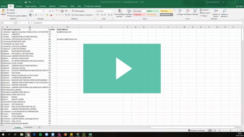
The example we prepared is the first proposed possibility: fetching company information in a contact export file.
Preparing your files
You should put your two Excel files in one Excel work book.
- The first tab should be the file where you want to execute your formula, in this case the contact file, where we want to insert the company information. The second tab, the company export in this case, should be the file where you will fetch the information from. You preferably give your tabs short, easy names. This will be useful in step 3 of the executing phase.
- The column order in your first tab doesn't matter. In your second tab, however, the common column in the two files/tabs should be the first one, column A. In our case this will be the company name.

Executing the VLookup
Go to the contact file or the first tab, name a new column after the information of the other tab you want to put there and start typing =VLookup. You will get a drop-down menu, where you need to choose the corresponding function.

Now you will see a formula where you will need to indicate the corresponding values:

- The lookup value will be the value of the common column 'Company name' in tab one on the same row as where you put your formula. Select the cell and put a dollar sign before the value of the cell, so B2 will become $B2. After selecting this cell, insert a semicolon or colon, as indicated in the formula, to get to the next part.
- We want to search this value in our second tab to be able to fetch the corresponding street and number of that company. This is why we select the whole table of the second tab as the range containing the return value. Ctrl+SHIFT+
 +
+ on Windows and Cmd+SHIFT++ on Mac selects your entire table right away if you want to save time.
 Now we return to the first tab. You will see that in your formula, the name of the second tab has changed to the name of the first tab. We will have to change 'Contacts' back to 'Companies' manually in this case. Moreover, we will have to put a dollar sign before the column and the row of the table range. This means, A1:F2243 will become $A$1:$F$2243. After selecting the lookup range, insert a semicolon or colon, as indicated in the formula, to get to the next part.
To select the return value, we go to our second tab, and have a look at in which column the needed information has been put. If the information needed is put in column B, the column number in our formula will be 2. If it is in column c, the number will be 3, and so on. One column number per formula can be put. If you want to fetch information from several columns, you will have to repeat this formula in your first tab. After selecting the column number with the return value, insert a semicolon or colon, as indicated in the formula, to get to the next part.
- Specify TRUE for approximate match or FALSE for an exact match; normally use cases related to Teamleader Focus will require 'FALSE'. Now you can close the brackets and let the magic work.
Example of what your formula will look like more or less in the end: - To apply this formula to all the other rows, double click on the tiny square of your formula cell:
Optional
If you want the return values of more than one column, you can drag the formula to the adjacent cells by clicking the tiny square and releasing it until you have selected as many columns as you want the return values of.
You will see however, that all cells now have the same return value. Click on the cell of the second column with a formula and change the column number as described in step 4. Repeat this respectively according to how many columns you want to retrieve information from.


Result
If all went well, you can get 3 types of output:
- The value you needed: in our example this is street+number
- An empty cell or a 0: this means the lookup value (company) has been found in tab 2, but the column with the return value for this specific lookup value is empty. In this case street and number have not been filled out
- #N/B: the lookup value (company) has not been found in tab 2

Remarks
- If you have several companies per contact, these companies will be in one cell in your contact export, separated by a comma. The VLookup-function, however, will regard "company1,company2" as the name of one single company. This means the VLookup function will return a response of #N/B, although these companies might be known in Teamleader Focus. Thus, for contacts with several companies, the return value should be checked in the second tab manually.
- If there is even a slightest difference in the common columns (Amazon vs Amaon), the status of #N/B will be returned.
- If you were wondering: the dollar signs in the formula are put to fix tables and/or rows. This is really important specifically for the lookup range. As you would copy the formula to the cells beneath, the lookup range would shift down too, which would make the lookup range smaller and would cause you to not get all return values available.